Additional Tools
Besides the main light curve extraction program (phot2lc) and the configuration program (photconfig), the phot2lc package also comes with a program for welding individual light curve files together (weldlc), and a program for generating light curve + periodogram plots using the .lc output files. This section provides information on how to use these tools.
addstar
A convenience function for adding new stars into the stars.dat file. This function has three required input arguments:
objectName    Name of object to add into stars.dat.
ra            Object Right Ascension in decimal degrees or HMS sexagesimal formats.
dec           Object Declination in decimal degrees or DMS sexagesimal formats.
Example usages with decimal degree versus HMSDMS sexagesimal coordinates:
addstar WDJ1944+4557  296.1330000  45.9647583
addstar WDJ1944+4557  "19 44 31.92"  "+45 57 53.13"
weldlc
A program designed for combining individual phot2lc light curve (.lc) files into a single light curve file. This program behaves much like WQED’s weld tool. Two command line options are available for this tool:
-f --infiles     Input files.
-b --bypass      Bypass the barycentric correction check and weld LC's anyways.
-o --outfile     Output filename.
weldlc will check the barycorr entries within each .lc file to make sure every light curve being welded has had barycentric time corrections applied. If one or more of the .lc files has barycorr = False, wildly will throw an error. If you know that your light curves are not all barycentric corrected and want to weld anyways, you can use the –bypass (-b) command to skip the check. An example usage would look like:
weldlc -f *.lc -o combined.lc
or
weldlc -f *.lc -o combined.lc --bypass
where *.lc would provide as input every .lc file within the current folder, and combined.lc would be the name of the resulting file with the combined light curve. A welded light curve file will have the same three data columns as an original .lc file, but different header information. An example header is given below:
# Object     = G117-B15A                     # Name of Object
# RA         = 09 24 15.27                   # Object Right Ascension
# Dec        = +35 16 51.3                   # Object Declination
# Date       = 2018-01-26                    # Mid-Exposure TDB Date at T0
# Time       = 05:14:54.080                  # Mid-Exposure TDB Time at T0
# BJED       = 2458144.718681479             # Mid-Exposure TDB JD at T0
# BaryCorr   = True                          # Whether the times are barycentric corrected
# WeldNum    = 2                             # Number of files welded
# Npoints    = 3905                          # Number of data points
# Tspan      = 1.14824075                    # Time spanned by data (days)
# WeldDate   = 2021-02-10 12:19:45.245       # File creation date
# Columns    = T-mid (s), Rel. Flux, Rel. Flux Error
quicklook
A program designed for quick analysis of phot2lc light curves and their periodograms. quicklook is also a command line tool with the following command line options:
-f --files      Input file(s) to perform quicklook on.
-s --save       Whether to save the quicklook plot.
-p --prewhiten  Whether to perform a pre-whitening sequence.
-l --lower      Lower frequency limit for pre-whitening search (micro-Hertz, default=500).
-u --upper      Upper frequency limit for pre-whitening search (micro-Hertz, default=100000).
-n --num        Maximum number of pre-whitening iterations (default=10).
-w --wqedlc     Whether the input file(s) are from WQED.
The -s, -p, and -w options don’t require an actual input. When they are called, they automatically pass a boolean value of TRUE to the quicklook program.
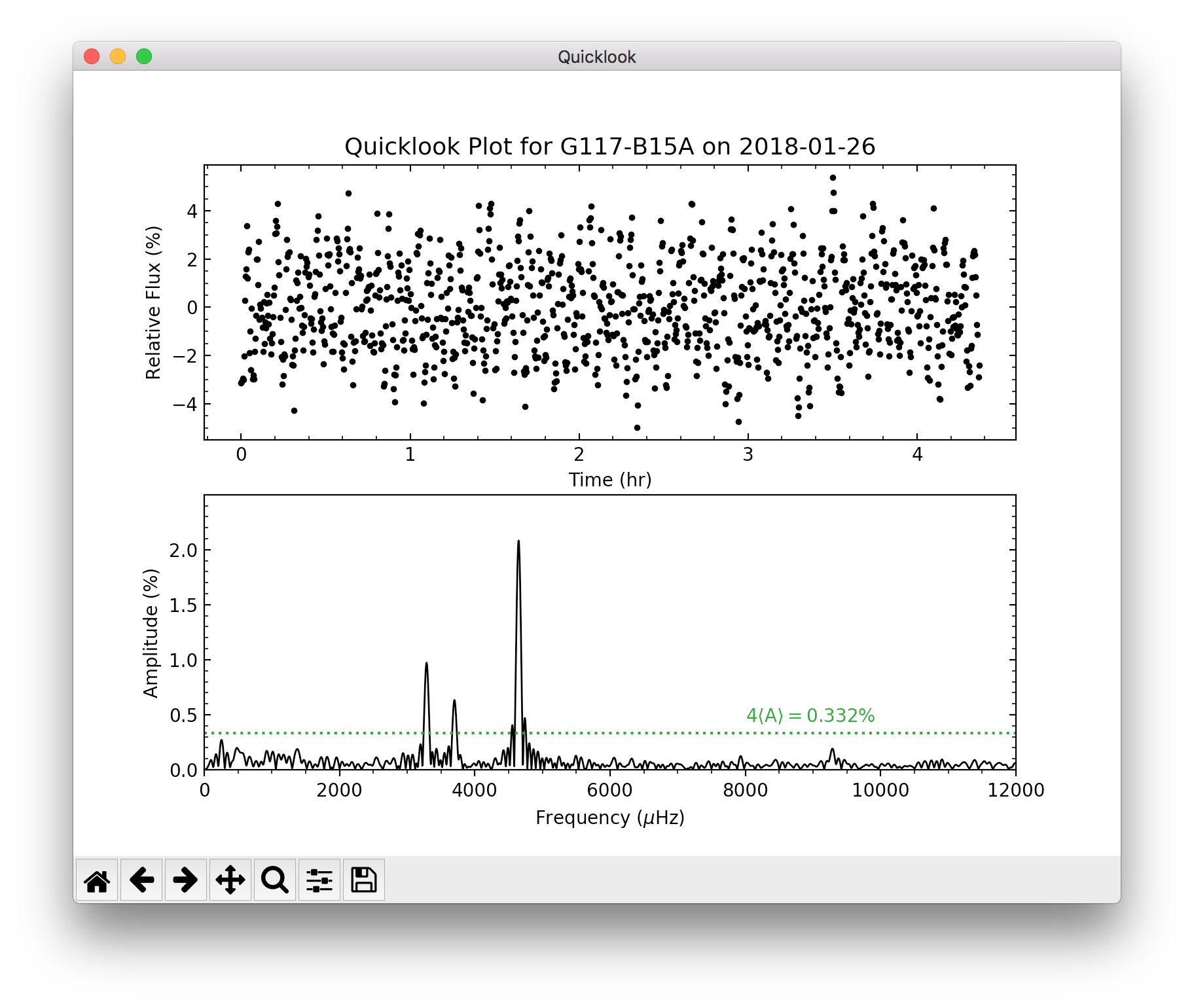
The only required command line input is -f, which you use to specify the file, or files, you wish to perform a quicklook for. Quicklook will always display the resulting plot, but will only save the plot if the -s option is specified. An example usage would be
quicklook -f *.lc
and the displayed plot would look like the following:
If you would like to perform a pre-whitening sequence to identify significant peaks in the periodogram, you need only specify the -p option. Pre-whitening is a procedure by which significant peaks in the periodogram are iteratively identified and then removed by subtracting a corresponding best-fit sinusoidal model from the light curve. Peaks are identified as significant if they rise above a significance threshold, which is defined in quicklook as four times the average periodogram amplitude, \(\langle 4\mathrm{A} \rangle\), between \(500\) and \(12{,}000\;\mu\mathrm{Hz}\). If a significant peak is found, its height and center are used as the initial guesses for a sinusoidal model’s amplitude and frequency, and a least squares fit (via LMFIT) is then performed to optimize those parameters. The resulting model is then subtracted from the light curve and a new periodogram of the residuals is calculated. This process repeats itself until no more significant peaks are found or until the maximum number of pre-whitening iterations set by -n is reached. Peaks are identified in order of decreasing amplitude.
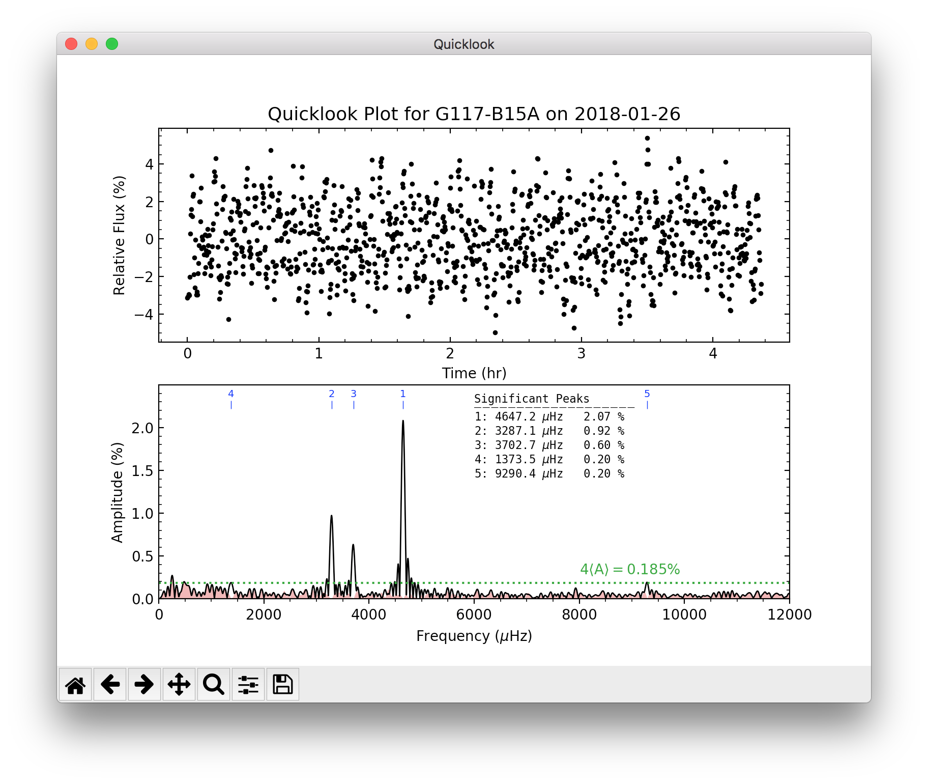
An example of using the pre-whitening option would look like:
quicklook -f *.lc -p
The resulting display (shown below) now has numbered markers labeling the locations of significant peaks, along with a table showing the best-fit frequency and amplitude of each peak from LMFIT. The black periodogram is before pre-whitening, while the red-shaded periodogram is after pre-whitening. The \(\langle 4\mathrm{A} \rangle\) threshold is representative of the red pre-whitened periodogram.
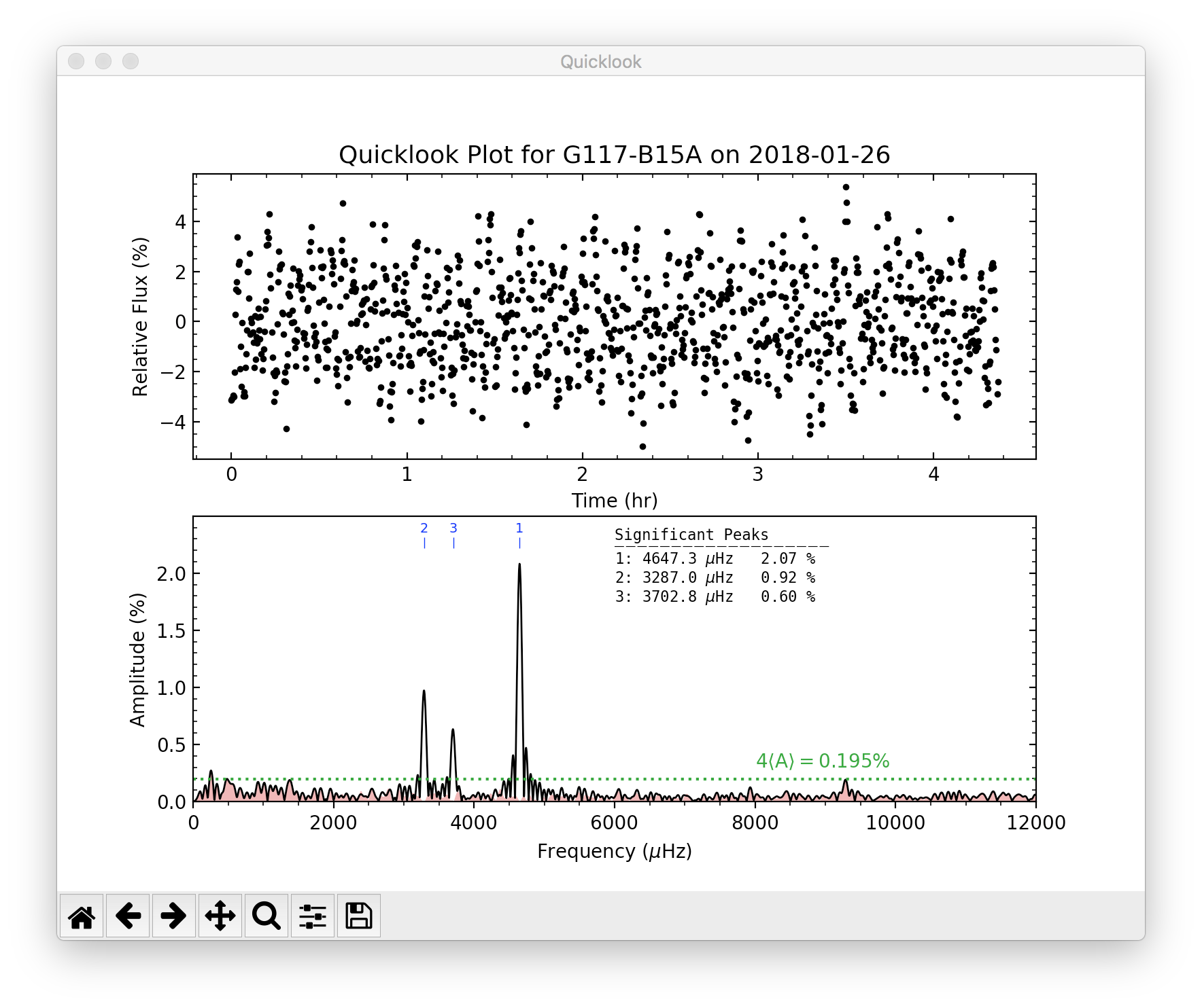
When the -p option is specified, the -l, -u, and -n options also become available. In the plot above, if for some reason you wanted to exclude peaks 4 and 5 from the pre-whitening procedure, you could do this by either limiting the frequency search range or by limiting the number of pre-whitening iterations. The commands would look like
quicklook -f *.lc -p -l 2000 -u 6000
or
quicklook -f *.lc -p -n 3
Either way, the resulting plot would look like:
Lastly, if you wish to use the quicklook function to analyze WQED light curve files, this is possible if you just specify the -w option:
quicklook -f *.lc1 -w